Machine Learning Algorithms in Python

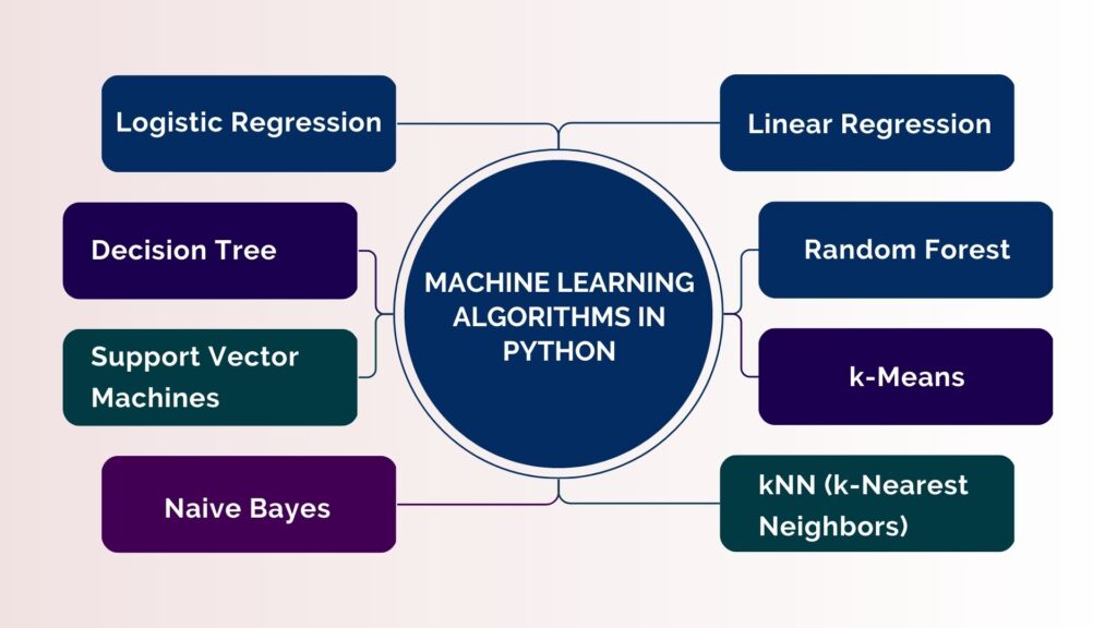
In this article, we will explore some of the most widely used machine learning algorithms that can be implemented in Python. We will cover a range of algorithms, including Linear Regression, Logistic Regression, Decision Trees, Support Vector Machines, Naive Bayes, kNN (k-Nearest Neighbors), k-Means, and Random Forest.

Linear Regression

Linear Regression is a simple yet powerful machine learning algorithm used for predicting a continuous output variable based on one or more input features. It is a type of supervised learning, where the algorithm is trained on a labeled dataset to learn the relationship between the input features and the output variable.

The goal of linear regression is to find the best-fitting straight line that can be used to make predictions on new data. The line is characterized by a slope (m) and an intercept (b), and the equation for a simple linear regression model is y = mx + b, where y is the output variable, x is the input feature, m is the slope, and b is the intercept.

To train a linear regression model in Python, we can use the Scikit-learn library, which provides a simple and efficient implementation of linear regression. We start by loading the dataset into a Pandas DataFrame and splitting it into training and testing sets. Then, we create an instance of the LinearRegression class and fit the model to the training data using the fit() method. Finally, we can use the predict() method to make predictions on the test data.

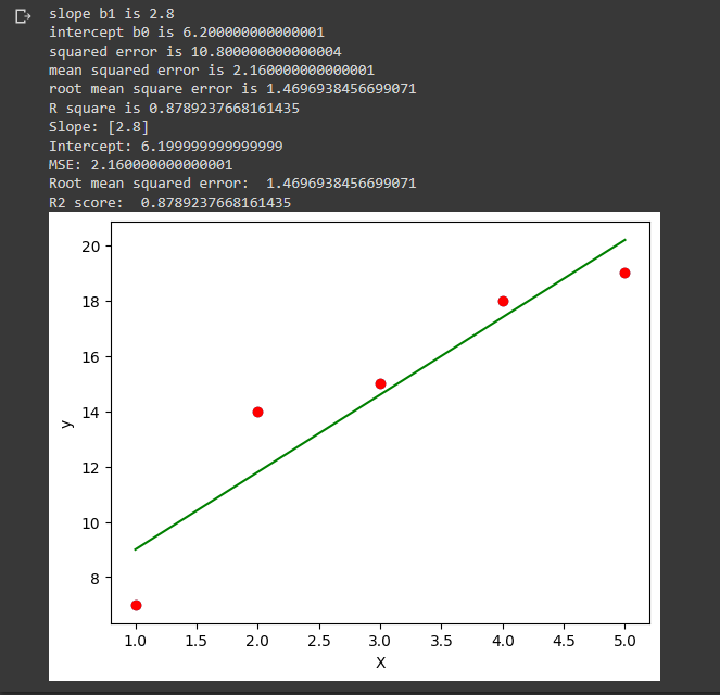
Let take a look at a simple example of Python Implementation in linear regression.

Step 1: Import all the necessary Libraries

import numpy as np
import matplotlib.pyplot as plt

from sklearn.linear_model import LinearRegression
from sklearn.metrics import mean_squared_error, r2_score
import statsmodels.api as sm

Step:2 Generate the date and Plot the given data points 

x = np.array([1,2,3,4,5])
y = np.array([7,14,15,18,19])
n = np.size(x)

x_mean = np.mean(x)
y_mean = np.mean(y)
x_mean,y_mean

Sxy = np.sum(x*y)- n*x_mean*y_mean
Sxx = np.sum(x*x)-n*x_mean*x_mean

b1 = Sxy/Sxx
b0 = y_mean-b1*x_mean
print('slope b1 is', b1)
print('intercept b0 is', b0)

plt.scatter(x,y)
plt.xlabel('Independent variable X')
plt.ylabel('Dependent variable y')
y_pred = b1 * x + b0

plt.scatter(x, y, color = 'red')
plt.plot(x, y_pred, color = 'green')
plt.xlabel('X')
plt.ylabel('y')

Step:3 Analyze the performance of the model by calculating mean squared error and R2

error = y - y_pred
se = np.sum(error**2)
print('squared error is', se)

mse = se/n
print('mean squared error is', mse)

rmse = np.sqrt(mse)
print('root mean square error is', rmse)

SSt = np.sum((y - y_mean)**2)
R2 = 1- (se/SSt)
print('R square is', R2)

Step:4 Use scikit library 

x = x.reshape(-1,1)
regression_model = LinearRegression()

# Fit the data(train the model)
regression_model.fit(x, y)

# Predict
y_predicted = regression_model.predict(x)

# model evaluation
mse=mean_squared_error(y,y_predicted)

rmse = np.sqrt(mean_squared_error(y, y_predicted))
r2 = r2_score(y, y_predicted)

# printing values
print('Slope:' ,regression_model.coef_)
print('Intercept:', regression_model.intercept_)
print('MSE:',mse)
print('Root mean squared error: ', rmse)
print('R2 score: ', r2)

Step:5 Run the above program

Logistic Regression

Logistic regression is a type of statistical model used to analyze the relationship between a dependent variable and one or more independent variables. It is a type of regression analysis commonly used to model binary outcomes (i.e., where the dependent variable has only two possible values, such as 0 or 1).

In logistic regression, the dependent variable is modeled as a function of one or more independent variables using a logistic function. The logistic function is an S-shaped curve that maps any real-valued input to a probability value between 0 and 1. The logistic function is defined as follows:

p(x) = 1 / (1 + exp(-z))

where p(x) is the probability of the dependent variable taking the value of 1, x is a vector of independent variables, z is a linear combination of the independent variables and their corresponding coefficients.

The logistic regression model estimates the coefficients of the independent variables to maximize the likelihood of observing the dependent variable values given the independent variables.

Logistic regression is widely used in various fields, including machine learning, social sciences, economics, and biomedical research, to model binary outcomes and to make predictions based on the values of the independent variables.

Decision Tree

A Decision Tree is a powerful machine learning algorithm used for both classification and regression tasks. It is a type of supervised learning, where the algorithm is trained on a labeled dataset to learn a series of if-then-else decision rules that can be used to make predictions on new data.

The basic idea behind decision trees is to divide the input space into a series of rectangles that correspond to different values of the input features. Each rectangle is associated with a prediction, and the algorithm uses a series of if-then-else rules to determine which rectangle a new data point belongs to.

To construct a decision tree in Python, we can use the Scikit-learn library, which provides a simple and efficient implementation of decision trees. We start by loading the dataset into a Pandas DataFrame and splitting it into training and testing sets. Then, we create an instance of the DecisionTreeClassifier class and fit the model to the training data using the fit() method. Finally, we can use the predict() method to make predictions on the test data.

Decision trees can be used for a wide range of applications, including predicting customer churn, identifying fraud, and diagnosing medical conditions. They are a powerful tool for making predictions based on complex decision rules and can provide valuable insights for decision-making in many industries.

Lets try Decision Tree using python

Step:1 Import required Package

import numpy as np
import pandas as pd
from sklearn.metrics import confusion_matrix
from sklearn.model_selection import train_test_split
from sklearn.tree import DecisionTreeClassifier
from sklearn.metrics import accuracy_score
from sklearn.metrics import classification_report

Step2: Import Data And Split the dataset into train and test

def importdata():
	balance_data = pd.read_csv(
'https://archive.ics.uci.edu/ml/machine-learning-'+
'databases/balance-scale/balance-scale.data',
	sep= ',', header = None)
	
	# Printing the dataswet shape
	print ("Dataset Length: ", len(balance_data))
	print ("Dataset Shape: ", balance_data.shape)
	
	# Printing the dataset obseravtions
	print ("Dataset: ",balance_data.head())
	return balance_data

def splitdataset(balance_data):

	# Separating the target variable
	X = balance_data.values[:, 1:5]
	Y = balance_data.values[:, 0]

	# Splitting the dataset into train and test
	X_train, X_test, y_train, y_test = train_test_split(
	X, Y, test_size = 0.3, random_state = 100)
	
	return X, Y, X_train, X_test, y_train, y_test

Step:3 Create function to train with giniIndex and entropy

def train_using_gini(X_train, X_test, y_train):

	clf_gini = DecisionTreeClassifier(criterion = "gini",
			random_state = 100,max_depth=3, min_samples_leaf=5)

	clf_gini.fit(X_train, y_train)
	return clf_gini
	
def tarin_using_entropy(X_train, X_test, y_train):

	clf_entropy = DecisionTreeClassifier(
			criterion = "entropy", random_state = 100,
			max_depth = 3, min_samples_leaf = 5)

	clf_entropy.fit(X_train, y_train)
	return clf_entropy


def prediction(X_test, clf_object):

	y_pred = clf_object.predict(X_test)
	print("Predicted values:")
	print(y_pred)
	return y_pred
	

Step:4 Calculate Accuracy

def cal_accuracy(y_test, y_pred):
	
	print("Confusion Matrix: ",
		confusion_matrix(y_test, y_pred))
	
	print ("Accuracy : ",
	accuracy_score(y_test,y_pred)*100)
	
	print("Report : ",
	classification_report(y_test, y_pred))

Step:5 Define and call the main function

def main():
		
	data = importdata()
	X, Y, X_train, X_test, y_train, y_test = splitdataset(data)
	clf_gini = train_using_gini(X_train, X_test, y_train)
	clf_entropy = tarin_using_entropy(X_train, X_test, y_train)
	
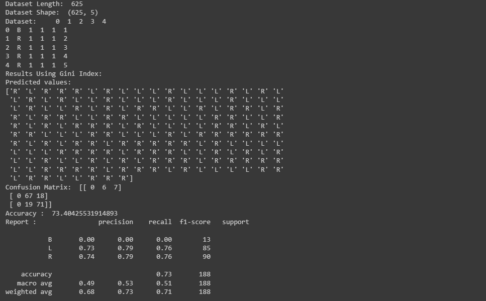
	print("Results Using Gini Index:")
		
	y_pred_gini = prediction(X_test, clf_gini)
	cal_accuracy(y_test, y_pred_gini)
	
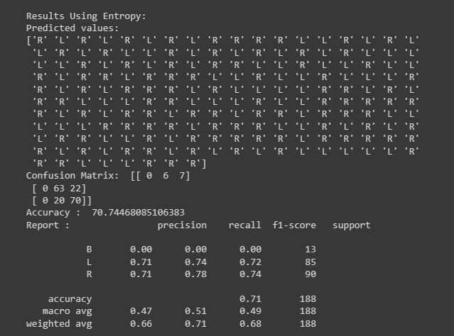
	print("Results Using Entropy:")
	y_pred_entropy = prediction(X_test, clf_entropy)
	cal_accuracy(y_test, y_pred_entropy)
	
	
# Calling main function
if __name__=="__main__":
	main()

Step:6 Run this python coding in your local file

Support Vector Machines (SVM)

Support Vector Machines (SVM) is a supervised machine learning algorithm used for classification, regression and outlier detection. SVM is a powerful and flexible algorithm that can handle both linear and non-linear data by transforming the data into higher dimensions.

In SVM, the algorithm tries to find the best boundary that separates the data into different classes. This boundary is called the hyperplane, which maximizes the margin between the classes. The margin is the distance between the hyperplane and the closest data points from each class.

SVM can handle binary classification and multi-class classification problems by using various techniques such as one-vs-one, one-vs-all, or multi-class SVM.

To find the optimal hyperplane, SVM optimizes a mathematical function called the objective function using the Lagrangian optimization technique. This function maximizes the margin between the classes while minimizing the classification error.

SVM is effective when the number of features is high, and the data points are separable. However, in cases where the data is not separable, SVM can use a technique called kernel trick to transform the data into a higher dimension, where it can be separated by a hyperplane. This technique involves using a kernel function, such as the radial basis function (RBF), to map the data to a higher dimensional space.

SVM is widely used in various fields such as image classification, text classification, bioinformatics, and finance, where it has shown excellent performance in classifying data into different categories.

Naive Bayes

Naive Bayes is a probabilistic machine learning algorithm based on Bayes’ theorem, which is used for classification and prediction tasks. The algorithm is called “naive” because it assumes that the features (independent variables) are conditionally independent of each other given the class label (dependent variable), even though this may not be the case in reality.

In Naive Bayes, the probability of each class label given the features is calculated using Bayes’ theorem:

P(y|x1, x2, …, xn) = P(x1, x2, …, xn|y) * P(y) / P(x1, x2, …, xn)

where y is the class label, x1, x2, …, xn are the features, P(y|x1, x2, …, xn) is the posterior probability of the class label given the features, P(x1, x2, …, xn|y) is the likelihood of the features given the class label, P(y) is the prior probability of the class label, and P(x1, x2, …, xn) is the evidence probability of the features.

Naive Bayes assumes that the features are conditionally independent of each other given the class label. This means that the likelihood of the features given the class label can be calculated as the product of the individual conditional probabilities of each feature given the class label:

P(x1, x2, …, xn|y) = P(x1|y) * P(x2|y) * … * P(xn|y)

The prior probability of the class label can be estimated from the training data, and the conditional probabilities of each feature given the class label can be estimated using various techniques such as maximum likelihood estimation or Bayesian estimation.

Naive Bayes is fast, simple to implement, and requires a small amount of training data compared to other classification algorithms. It is often used in text classification tasks such as spam detection, sentiment analysis, and document classification, but can also be used in other classification problems such as image classification, medical diagnosis, and fraud detection.

kNN (k-Nearest Neighbors)

kNN, short for k-Nearest Neighbors, is a type of supervised machine learning algorithm used for classification and regression problems.

The kNN algorithm works by comparing a new input data point to the k closest training data points in the feature space. The feature space is a mathematical representation of the input data where each feature (also known as predictor or independent variable) is a dimension.

In the case of classification problems, the output is a categorical variable. The algorithm assigns the class label that is most frequent among the k closest neighbors. For example, if we have a set of labeled data points that belong to two classes (e.g., “cat” and “dog”), and we want to classify a new data point, we first identify the k nearest neighbors to the new data point in the feature space. Then, we assign the class label that is most frequent among those k neighbors to the new data point.

In the case of regression problems, the output is a continuous variable. The algorithm predicts the value of the new data point by averaging the values of the k closest neighbors. For example, if we have a set of labeled data points that represent the price of houses based on their square footage, and we want to predict the price of a new house based on its square footage, we first identify the k nearest neighbors to the new data point in the feature space. Then, we predict the price of the new house by averaging the prices of those k neighbors.

The value of k is a hyperparameter that needs to be tuned. A small value of k can lead to overfitting, where the algorithm assigns too much weight to the noise in the data, while a large value of k can lead to underfitting, where the algorithm does not capture the underlying patterns in the data. Therefore, the value of k needs to be chosen carefully based on the complexity of the problem and the size of the dataset.

k-Means

k-Means is an unsupervised machine learning algorithm used for clustering data points based on their similarity in the feature space. The algorithm tries to partition a set of n data points into k clusters, where each data point belongs to the cluster whose centroid is the closest to it in the feature space.

The k-Means algorithm works by first randomly selecting k initial centroids, which are the center points of each cluster. Then, for each data point in the dataset, the algorithm calculates the distance between the point and each of the k centroids, and assigns the point to the cluster whose centroid is the closest to it. This step creates k clusters.

Next, the algorithm calculates the new centroids for each cluster as the mean of all the data points assigned to that cluster. The algorithm then repeats the previous step until the centroids no longer change significantly or a maximum number of iterations is reached.

The value of k is a hyperparameter that needs to be determined beforehand. The value of k can be chosen based on the problem domain or by using a technique such as the elbow method, which plots the percentage of variance explained as a function of the number of clusters and looks for the “elbow” point where adding more clusters does not significantly improve the model.

One drawback of the k-Means algorithm is that it is sensitive to the initial placement of the centroids. Different random initializations may result in different cluster assignments and centroids. To address this, the algorithm is often run multiple times with different initializations, and the result with the lowest sum of squared distances between data points and their assigned centroids is chosen.

Random Forest

Random Forest is a supervised machine learning algorithm used for classification, regression, and other tasks such as outlier detection. It is an ensemble learning method that combines multiple decision trees to make a prediction.

The Random Forest algorithm works by building a multitude of decision trees at training time. Each tree is trained on a random subset of the training data and a random subset of the features (predictors/independent variables) at each split. This random selection of features and data points is what makes the algorithm “random” and helps reduce overfitting.

During prediction, each tree in the forest independently produces a prediction, and the final prediction is the majority vote (classification) or the average (regression) of the predictions from all the trees in the forest.

Random Forest has several advantages over a single decision tree, including better generalization performance, higher accuracy, and reduced risk of overfitting. It also handles missing data well and can handle both categorical and continuous data.

The hyperparameters of the Random Forest algorithm include the number of trees in the forest, the maximum depth of each tree, and the number of features to consider at each split. These hyperparameters can be tuned using techniques such as cross-validation to optimize the performance of the algorithm.

One disadvantage of Random Forest is that it can be computationally expensive and memory-intensive, especially for large datasets.

This article is to help readers gain a better understanding of Machine Learning Algorithms in Python. We trust that it has been helpful to you. Please feel free to share your thoughts and feedback in the comment section below.